ArangoDB Graphs
First Steps with Graphs
A Graph consists of vertices and edges. Edges are stored as documents in edge collections. A vertex can be a document of a document collection or of an edge collection (so edges can be used as vertices).
Which collections are used within a named graph is defined via edge definitions. They describe which edge collections connect which vertex collections. A named graph can contain more than one edge definition, at least one is needed. Graphs allow you to structure your models in line with your domain and group them logically in collections and giving you the power to query them in the same graph queries.
New to graphs? Take our free graph course for freshers and get from zero knowledge to advanced query techniques.
Coming from a relational background - what’s a graph?
In SQL you commonly have the construct of a relation table to store n:m relations between two data tables.
An edge collection is somewhat similar to these relation tables; vertex collections resemble the data tables with the objects to connect.
While simple graph queries with fixed number of hops via the relation table may be doable in SQL with several nested joins,
graph databases can handle an arbitrary number of these hops over edge collections - this is called traversal.
Also edges in one edge collection may point to several vertex collections.
Its common to have attributes attached to edges, i.e. a label naming this interconnection.
Edges have a direction, with their relations _from and _to pointing from one document to another document stored in vertex collections.
In queries you can define in which directions the edge relations may be followed (OUTBOUND: _from → _to, INBOUND: _from ← _to, ANY: _from ↔ _to).
Supported Graph Algorithms
- Traversal
- following edges in outbound, inbound, or any direction
- variable traversal depth between a defined minimum and maximum
- breadth-first, depth-first, and weighted traversals
- optionally with prune conditions
- Shortest Path
- All Shortest Paths
- k Shortest Paths
- k Paths
- Distributed Iterative Graph Processing (Pregel)
- Page Rank
- Seeded Page Rank
- Single-Source Shortest Path (SSSP)
- Connected Components
- Weakly Connected Components (WCC)
- Strongly Connected Components (SCC)
- Hyperlink-Induced Topic Search (HITS)
- Effective Closeness Vertex Centrality
- LineRank Vertex Centrality
- Label Propagation Community Detection
- Speaker-Listener Label Propagation (SLPA) Community Detection
Named Graphs
Named graphs are completely managed by ArangoDB, and thus also visible in the web interface. They use the full spectrum of ArangoDB’s graph features. You may access them via several interfaces.
- AQL Graph Operations with several flavors:
- AQL Traversals on both named and anonymous graphs
- AQL Shortest Path on both named and anonymous graph
- JavaScript General Graph implementation, as you may use it in Foxx Services
- Graph Management; creating & manipulating graph definitions; inserting, updating and deleting vertices and edges into graphs
- Graph Functions for working with edges and vertices, to analyze them and their relations
- JavaScript SmartGraph implementation, for scalable graphs
- SmartGraph Management; creating & manipulating SmartGraph definitions; Differences to General Graph
- RESTful General Graph interface used to implement graph management in client drivers
Manipulating collections of named graphs with regular document functions
The underlying collections of the named graphs are still accessible using the standard methods for collections. However the graph module adds an additional layer on top of these collections giving you the following guarantees:
- All modifications are executed transactional
- If you delete a vertex all edges referring to this vertex will be deleted too
- If you insert an edge it is checked if the edge matches the edge definitions
Your edge collections will only contain valid edges and you will never have loose ends. These guarantees are lost if you access the collections in any other way than the graph module, so if you delete documents from your vertex collections directly, the edges pointing to them will be remain in place.
Existing inconsistencies in your data will not be corrected when you create a named graph. Therefore, make sure you start with sound data as otherwise there could be dangling edges after all. The graph module guarantees to not introduce new inconsistencies only.
Anonymous graphs
Sometimes you may not need all the powers of named graphs, but some of its bits may be valuable to you. You may use anonymous graphs in the traversals and in the Working with Edges chapter. Anonymous graphs don’t have edge definitions describing which vertex collection is connected by which edge collection. The graph model has to be maintained in the client side code. This gives you more freedom than the strict named graphs.
- AQL Graph Operations are available for both, named and anonymous graphs:
When to choose anonymous or named graphs
As noted above, named graphs ensure graph integrity, both when inserting or removing edges or vertices. So you won’t encounter dangling edges, even if you use the same vertex collection in several named graphs. This involves more operations inside the database which come at a cost. Therefore anonymous graphs may be faster in many operations. So this question may be narrowed down to: ‘Can I afford the additional effort or do I need the warranty for integrity?’.
Multiple edge collections vs. FILTERs on edge document attributes
If you want to only traverse edges of a specific type, there are two ways to achieve this. The first would be
an attribute in the edge document - i.e. type, where you specify a differentiator for the edge -
i.e. "friends", "family", "married" or "workmates", so you can later FILTER e.type = "friends"
if you only want to follow the friend edges.
Another way, which may be more efficient in some cases, is to use different edge collections for different
types of edges, so you have friend_edges, family_edges, married_edges and workmate_edges as collection names.
You can then configure several named graphs including a subset of the available edge and vertex collections -
or you use anonymous graph queries, where you specify a list of edge collections to take into account in that query.
To only follow friend edges, you would specify friend_edges as sole edge collection.
Both approaches have advantages and disadvantages. FILTER operations on edge attributes will do comparisons on
each traversed edge, which may become CPU-intense. When not finding the edges in the first place because of the
collection containing them is not traversed at all, there will never be a reason to actually check for their
type attribute with FILTER.
The multiple edge collections approach is limited by the number of collections that can be used simultaneously in one query. Every collection used in a query requires some resources inside of ArangoDB and the number is therefore limited to cap the resource requirements. You may also have constraints on other edge attributes, such as a hash index with a unique constraint, which requires the documents to be in a single collection for the uniqueness guarantee, and it may thus not be possible to store the different types of edges in multiple edge collections.
So, if your edges have about a dozen different types, it’s okay to choose the collection approach, otherwise
the FILTER approach is preferred. You can still use FILTER operations on edges of course. You can get rid
of a FILTER on the type with the former approach, everything else can stay the same.
Which part of my data is an Edge and which a Vertex?
The main objects in your data model, such as users, groups or articles, are usually considered to be vertices. For each type of object, a document collection (also called vertex collection) should store the individual entities. Entities can be connected by edges to express and classify relations between vertices. It often makes sense to have an edge collection per relation type.
ArangoDB does not require you to store your data in graph structures with edges and vertices, you can also decide
to embed attributes such as which groups a user is part of, or _ids of documents in another document instead of
connecting the documents with edges. It can be a meaningful performance optimization for 1:n relationships, if
your data is not focused on relations and you don’t need graph traversal with varying depth. It usually means
to introduce some redundancy and possibly inconsistencies if you embed data, but it can be an acceptable tradeoff.
Vertices
Let’s say we have two vertex collections, Users and Groups. Documents in the Groups collection contain the attributes
of the Group, i.e. when it was founded, its subject, an icon URL and so on. Users documents contain the data specific to a
user - like all names, birthdays, Avatar URLs, hobbies…
Edges
We can use an edge collection to store relations between users and groups. Since multiple users may be in an arbitrary
number of groups, this is an m:n relation. The edge collection can be called UsersInGroups with i.e. one edge
with _from pointing to Users/John and _to pointing to Groups/BowlingGroupHappyPin. This makes the user John
a member of the group Bowling Group Happy Pin. Attributes of this relation may contain qualifiers to this relation,
like the permissions of John in this group, the date when John joined the group etc.

So roughly put, if you use documents and their attributes in a sentence, nouns would typically be vertices, verbs become the edges. You can see this in the knows graph below:
Alice knows Bob, who in term knows Charlie.
Advantages of this approach
Graphs give you the advantage of not just being able to have a fixed number of m:n relations in a row, but an arbitrary number. Edges can be traversed in both directions, so it’s easy to determine all groups a user is in, but also to find out which members a certain group has. Users could also be interconnected to create a social network.
Using the graph data model, dealing with data that has lots of relations stays manageable and can be queried in very flexible ways, whereas it would cause headache to handle it in a relational database system.
Backup and restore
For sure you want to have backups of your graph data, you can use arangodump to create the backup, and arangorestore to restore a backup into a new ArangoDB. You should however note that:
- you need the system collection
_graphsif you backup named graphs. - you need to backup the complete set of all edge and vertex collections your graph consists of. Partial dump/restore may not work.
Managing graphs
By default you should use the interface your driver provides to manage graphs.
This is i.e. documented in Graphs-Section of the ArangoDB Java driver.
Example Graphs
ArangoDB comes with a set of easily graspable graphs that are used to demonstrate the APIs.
You can use the add samples tab in the create graph window in the web interface, or load the module @arangodb/graph-examples/example-graph in arangosh and use it to create instances of these graphs in your ArangoDB.
Once you’ve created them, you can inspect them in the web interface - which was used to create the pictures below.
You can easily look into the innards of this script for reference about how to manage graphs programmatically.
The Knows_Graph
A set of persons knowing each other:
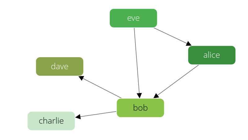
The knows graph consists of one vertex collection persons connected via one edge collection knows.
It will contain five persons Alice, Bob, Charlie, Dave and Eve.
We will have the following directed relations:
- Alice knows Bob
- Bob knows Charlie
- Bob knows Dave
- Eve knows Alice
- Eve knows Bob
This is how we create it, inspect its vertices and edges, and drop it again:
Note: with the default “Search Depth” of 2 of the graph viewer you may not see all edges of this graph.
The Social Graph
A set of persons and their relations:
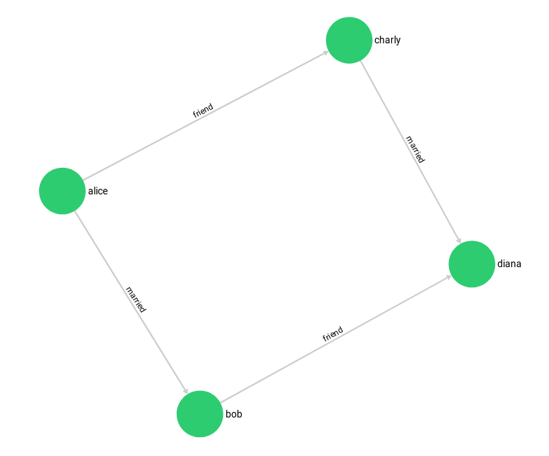
This example has female and male persons as vertices in two vertex collections - female and male. The edges are their connections in the relation edge collection.
This is how we create it, inspect its vertices and edges, and drop it again:
The City Graph
A set of european cities, and their fictional traveling distances as connections:
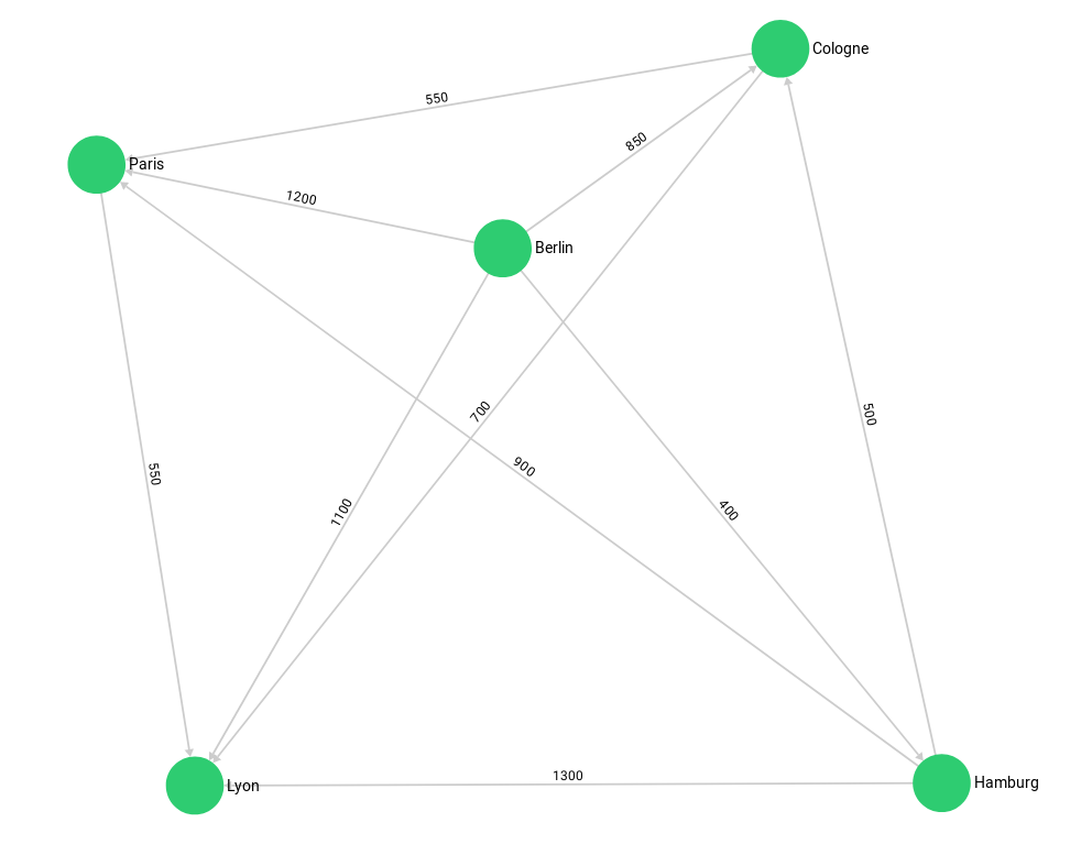
The example has the cities as vertices in several vertex collections - germanCity and frenchCity. The edges are their interconnections in several edge collections french / german / international Highway. This is how we create it, inspect its edges and vertices, and drop it again:
The Traversal Graph
This graph was designed to demonstrate filters in traversals. It has some labels to filter on it.
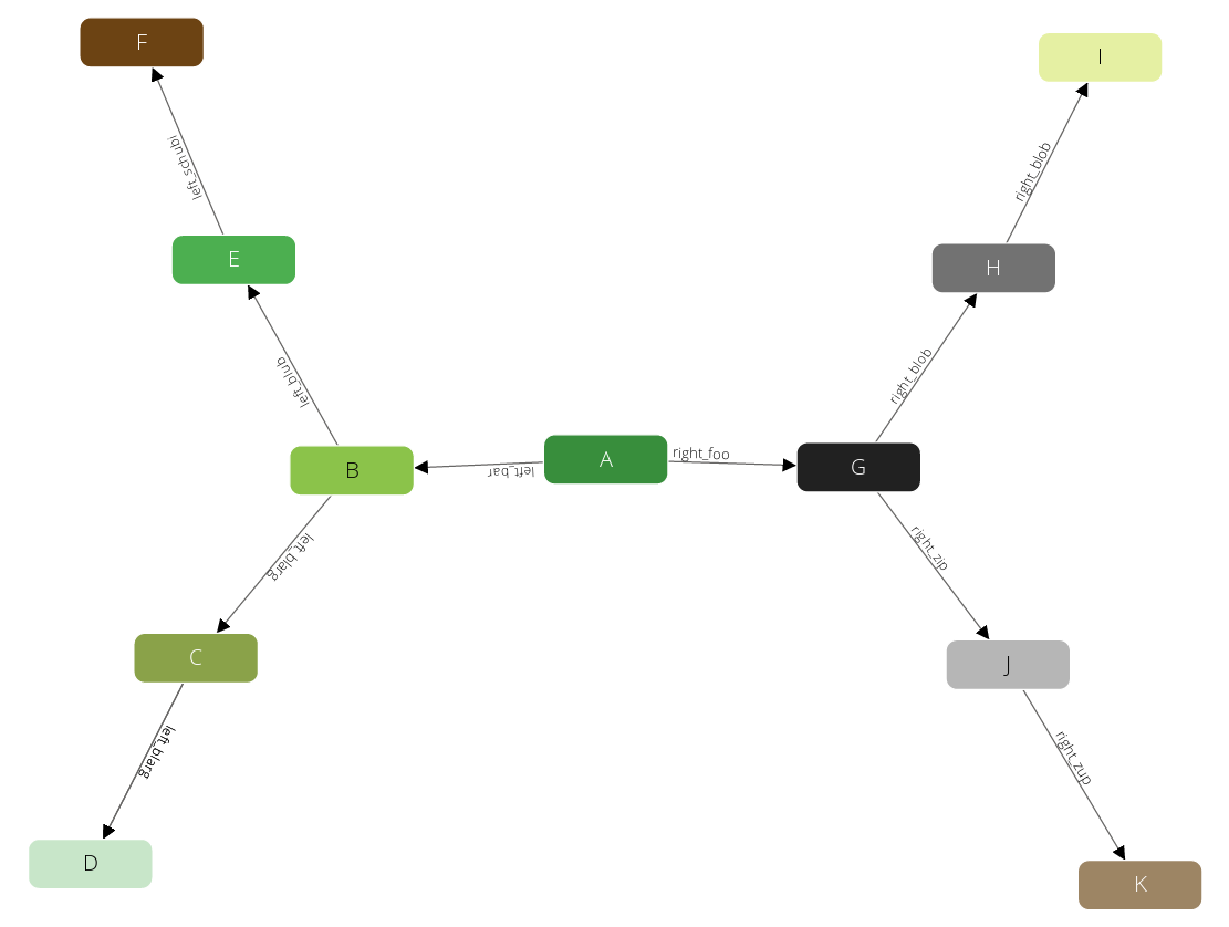
The example has all its vertices in the circles collection, and an edges edge collection to connect them. Circles have unique numeric labels. Edges have two boolean attributes (theFalse always being false, theTruth always being true) and a label sorting B - D to the left side, G - K to the right side. Left and right side split into Paths - at B and G which are each direct neighbours of the root-node A. Starting from A the graph has a depth of 3 on all its paths.
Note: with the default “Search Depth” of 2 of the graph viewer you may not see all nodes of this graph.
The k Shortest Paths Graph
The vertices in this graph are train stations of cities in Europe and North America and the edges represent train connections between them, with the travel time for both directions as edge weight.

See the k Shortest Paths page for query examples.
The World Graph
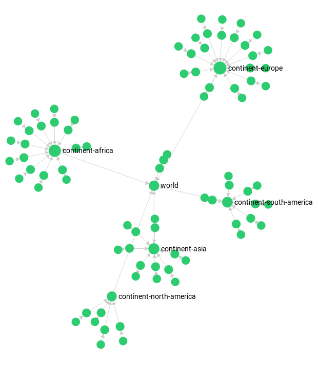
The world country graph structures its nodes like that: world → continent → country → capital. In some cases edge directions aren’t forward (therefore it will be displayed disjunct in the graph viewer). It has two ways of creating it. One using the named graph utilities (worldCountry), one without (worldCountryUnManaged). It is used to demonstrate raw traversal operations.
The Mps Graph
This graph was created to demonstrate a use case of the shortest path algorithm. Even though the algorithm can only determine one shortest path, it is possible to return multiple shortest paths with two separate queries. Therefore the graph is named after the multiple path search use case.
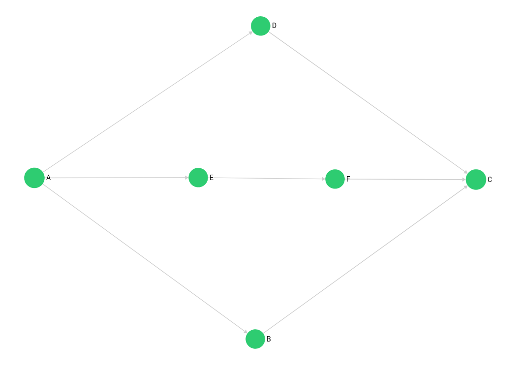
The example graph consists of vertices in the mps_verts collection and edges in the mps_edges collection. It is a simple traversal graph with start node A and end node C.
This is how we create it, inspect its vertices and edges, and drop it again:
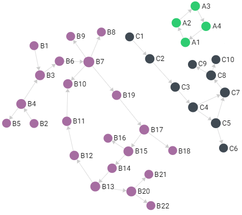
The Connected Components Graph
A small example graph comprised of components (vertices) and connections
(edges). Good for trying out Pregel algorithms such as Weakly Connected
Components (WCC).
Also see:
Higher volume graph examples
All of the above examples are rather small so they are easier to comprehend and can demonstrate the way the functionality works. There are however several datasets freely available on the web that are a lot bigger. We collected some of them with import scripts so you may play around with them. Another huge graph is the Pokec social network from Slovakia that we used for performance testing on several databases; You will find importing scripts etc. in this blogpost.

