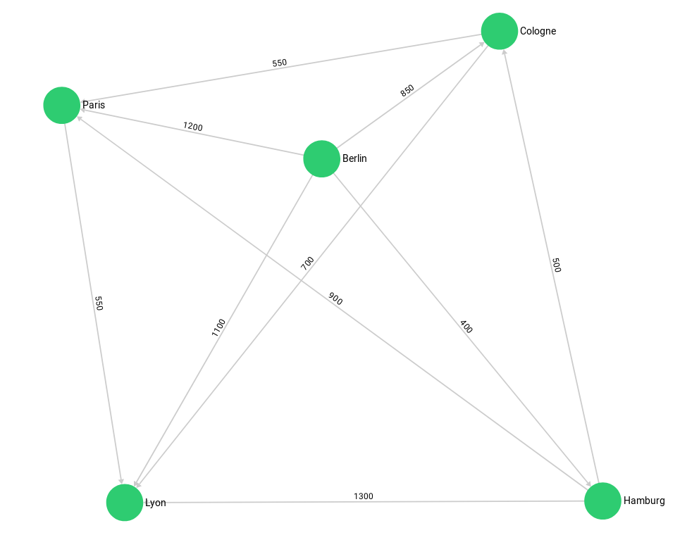
Combining Graph Traversals
Finding the start vertex via a geo query
Our first example will locate the start vertex for a graph traversal via a geo index.
We use the city graph and its geo indexes:

arangosh> var examples = require("@arangodb/graph-examples/example-graph.js");
arangosh> var g = examples.loadGraph("routeplanner");
We search all german cities in a range of 400 km around the ex-capital Bonn: Hamburg and Cologne.
We won’t find Paris since its in the frenchCity collection.
FOR startCity IN germanCity
    FILTER GEO_DISTANCE(@bonn, startCity.geometry) < @radius
      RETURN startCity._key
Bind Parameters:
{
  "bonn": [
    7.0998,
    50.734
  ],
  "radius": 400000
}
Result:
[
  "Cologne",
  "Hamburg"
]
Let’s revalidate that the geo indexes are actually used:
FOR startCity IN germanCity
    FILTER GEO_DISTANCE(@bonn, startCity.geometry) < @radius
      RETURN startCity._key
Bind Parameters:
{
  "bonn": [
    7.0998,
    50.734
  ],
  "radius": 400000
}
Explain:
Query String (119 chars, cacheable: true):
   FOR startCity IN germanCity
     FILTER GEO_DISTANCE(@bonn, startCity.geometry) < @radius
       RETURN startCity._key


Execution plan:
 Id   NodeType          Est.   Comment
  1   SingletonNode        1   * ROOT
  7   IndexNode            0     - FOR startCity IN germanCity   /* geo index scan, index scan + document lookup (projections: `_key`) */
  5   CalculationNode      0       - LET #3 = startCity.`_key`   /* attribute expression */   /* collections used: startCity : germanCity */
  6   ReturnNode           0       - RETURN #3

Indexes used:
 By   Name                      Type   Collection   Unique   Sparse   Cache   Selectivity   Fields           Stored values   Ranges
  7   idx_1762249842001707011   geo    germanCity   false    true     false           n/a   [ `geometry` ]   [  ]            (GEO_DISTANCE([ 7.0998, 50.734 ], startCity.`geometry`) < 400000)

Optimization rules applied:
 Id   RuleName
  1   move-calculations-up
  2   move-filters-up
  3   move-calculations-up-2
  4   move-filters-up-2
  5   geo-index-optimizer
  6   remove-unnecessary-calculations-2
  7   reduce-extraction-to-projection

44 rule(s) executed, 1 plan(s) created, peak mem [b]: 0, exec time [s]: 0.00020
And now combine this with a graph traversal:
FOR startCity IN germanCity
    FILTER GEO_DISTANCE(@bonn, startCity.geometry) < @radius
      FOR v, e, p IN 1..1 OUTBOUND startCity
        GRAPH 'routeplanner'
      RETURN {startcity: startCity._key, traversedCity: v._key}
Bind Parameters:
{
  "bonn": [
    7.0998,
    50.734
  ],
  "radius": 400000
}
Result:
[
  {
    "startcity": "Cologne",
    "traversedCity": "Paris"
  },
  {
    "startcity": "Cologne",
    "traversedCity": "Lyon"
  },
  {
    "startcity": "Hamburg",
    "traversedCity": "Lyon"
  },
  {
    "startcity": "Hamburg",
    "traversedCity": "Paris"
  },
  {
    "startcity": "Hamburg",
    "traversedCity": "Cologne"
  }
]
The geo index query returns us startCity (Cologne and Hamburg) which we then use as starting point for our graph traversal.
For simplicity we only return their direct neighbours. We format the return result so we can see from which startCity the traversal came.
Alternatively we could use a LET statement with a subquery to group the traversals by their startCity efficiently:
FOR startCity IN germanCity
    FILTER GEO_DISTANCE(@bonn, startCity.geometry) < @radius
      LET oneCity = (
        FOR v, e, p IN 1..1 OUTBOUND startCity
          GRAPH 'routeplanner' RETURN v._key
      )
        RETURN {startCity: startCity._key, connectedCities: oneCity}
Bind Parameters:
{
  "bonn": [
    7.0998,
    50.734
  ],
  "radius": 400000
}
Result:
[
  {
    "startCity": "Cologne",
    "connectedCities": [
      "Paris",
      "Lyon"
    ]
  },
  {
    "startCity": "Hamburg",
    "connectedCities": [
      "Lyon",
      "Paris",
      "Cologne"
    ]
  }
]
Finally, we clean up again:
arangosh> examples.dropGraph("routeplanner");


